Reading experimental data files
CGMF python utilities come with the capability of reading experimental data sets saved in JSON (JavaScript Object Notation) format. Simple routines exist to read and plot experimental data sets for a given physical quantity.
[1]:
### initializations and import libraries
import numpy as np
import matplotlib.pyplot as plt
import matplotlib.gridspec as gridspec
%matplotlib inline
%pylab inline

#import fission.py #-- my own library
sys.path.append('/Users/talou/git/evaluation-tools/')
import fission as fission
#import fissionHistories as fh
Populating the interactive namespace from numpy and matplotlib
[2]:
### rcParams are the default parameters for matplotlib
import matplotlib as mpl

print ("Matplotbib Version: ", mpl.__version__)

mpl.rcParams['font.size'] = 18
mpl.rcParams['font.family'] = 'Helvetica', 'serif'
#mpl.rcParams['font.color'] = 'darkred'
mpl.rcParams['font.weight'] = 'normal'

mpl.rcParams['axes.labelsize'] = 18.
mpl.rcParams['xtick.labelsize'] = 18.
mpl.rcParams['ytick.labelsize'] = 18.
mpl.rcParams['lines.linewidth'] = 2.

font = {'family' : 'serif',
        'color'  : 'darkred',
        'weight' : 'normal',
        'size'   : 18,
        }

mpl.rcParams['xtick.major.pad']='10'
mpl.rcParams['ytick.major.pad']='10'

mpl.rcParams['image.cmap'] = 'inferno'
Matplotbib Version: 2.0.0
Reading a JSON file
You can read a JSON-formatted file and save its content in a JSON object:
[3]:
exp = fission.readJSONDataFile ("/Users/talou/git/cgmf/exp/data-98252sf.json")
Listing the contents of the ‘exp’ object:
[4]:
fission.listExperimentalData(exp)
YA         |  F.-J. Hambsch, S. Oberstedt, P. Siegler, J. van Arle, R. Vogt, 1997
YA         |  C. Budtz-Joergensen and H.-H. Knitter, 1988
YA         |  A. Gook, F.-J. Hambsch, M. Vidali, 2014
YA         |  Sh. Zeynalov, F.-J.Hambsch, et al., 2011
YZ         |  Wahl, 1987
TKEA       |  Gook, 2014
SIGTKEA    |  A. Gook et al., 2014
Pnu        |  P. Santi and M. Miller, 2008
PFNS       |  W. Mannhart, 1989
PFNS2      |  W. Mannhart, 1989
nubarA     |  Vorobyev et al., 2004
EcmA       |  Budtz-Jorgensen and Knitter, 1988
nubarTKE   |  A. Gook, F.-J. Hambsch, M. Vidali, 2014
nubarTKE_A110 |  A. Gook, F.-J. Hambsch, M. Vidali, 2014
nubarTKE_A122 |  A. Gook, F.-J. Hambsch, M. Vidali, 2014
nubarTKE_A130 |  A. Gook, F.-J. Hambsch, M. Vidali, 2014
nubarTKE_A142 |  A. Gook, F.-J. Hambsch, M. Vidali, 2014
nLF        |  A. Skarsvag and K. Bergheim, 1963
nLF        |  H. R. Bowman, S. G. Thompson, J. C. D. Milton, and W. J. Swiatecki, 1962
nLF-A122   |  A. Gook, F.-J. Hambsch, M. Vidali, 2014
nLF-A96    |  A. Gook, F.-J. Hambsch, M. Vidali, 2014
nLF-A107   |  A. Gook, F.-J. Hambsch, M. Vidali, 2014
nLF-A116   |  A. Gook, F.-J. Hambsch, M. Vidali, 2014
nn         |  Pozzi et al., 2014
Pnug       |  A. Oberstedt, R. Billnert, F.-J. Hambsch, S. Oberstedt, et al., 2015
PFGS       |  Verbinski, 1973
PFGS1      |  R. Billnert, F.-J. Hambsch, A. Oberstedt, and S. Oberstedt, 2013
PFGS2      |  R. Billnert, F.-J. Hambsch, A. Oberstedt, and S. Oberstedt, 2013
multiplicityRatio |  T. Wang et al., 2016
PFGSvsA    |  A.Hotzel, P.Thirolf, Ch.Ender, D.Schwalm, M.Mutterer, P.Singer, M.Klemens, J.P.Theobald, M.Hesse, F.Goennenwein, H.v.d.Ploeg, 1996
You can limit the output to just one type of data. For instance, if one is only interested in checking out the mass yields, we would type:
[5]:
fission.listExperimentalData (exp, quantity="YA")
YA         |  F.-J. Hambsch, S. Oberstedt, P. Siegler, J. van Arle, R. Vogt, 1997
YA         |  C. Budtz-Joergensen and H.-H. Knitter, 1988
YA         |  A. Gook, F.-J. Hambsch, M. Vidali, 2014
YA         |  Sh. Zeynalov, F.-J.Hambsch, et al., 2011
Plotting Experimental Data
The fission package provides a simple routine to add experimental data to your plots.
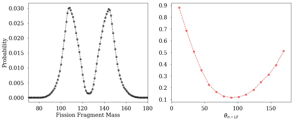
[6]:
fig=figure(figsize(14,6))

plt.subplot(1,2,1)
fission.plotExperimentalData(exp, quantity='YA',author="Gook")
plt.xlim(70,180)
plt.xlabel("Fission Fragment Mass")
plt.ylabel("Probability")

plt.subplot(1,2,2)
fission.plotExperimentalData(exp, quantity='nLF',author="Bowman",format="ro--")
plt.xlim(0,180)
plt.xlabel(r"$\theta_{n-{\rm LF}}$")

plt.tight_layout()
plt.show()
[ ]: