Reading CGMF Fission Yields

### initializations and import libraries
import numpy as np
import matplotlib.pyplot as plt
import matplotlib.gridspec as gridspec
%matplotlib inline
%pylab inline

import fission

Populating the interactive namespace from numpy and matplotlib

CGMF can be used to generate pre-neutron emission fission fragment yields in charge, mass, kinetic energy, excitation energy, spin, and parity. Those yields \(Y(Z,A,KE,U,J,\pi)\) set the initial conditions for the decay of the fragments by emission of prompt neutrons and \(\gamma\) rays.

To create an output file containing such yields, CGMF can be used with a negative number of events using the ‘-n’ option:

./cgmf.x -i 98252 -e 0.0 -n -1000000

It creates an output file that can easily be read:

yields = fission.readFragmentYieldsFromCGMF ("/Users/talou/git/cgmf/src/yields.1m.dat")

Sorting the data by mass, charge, etc, is trivial:

Z  = yields[:,0]
A  = yields[:,1]
KE = yields[:,2]
U  = yields[:,3]
J  = yields[:,4]
p  = yields[:,5]

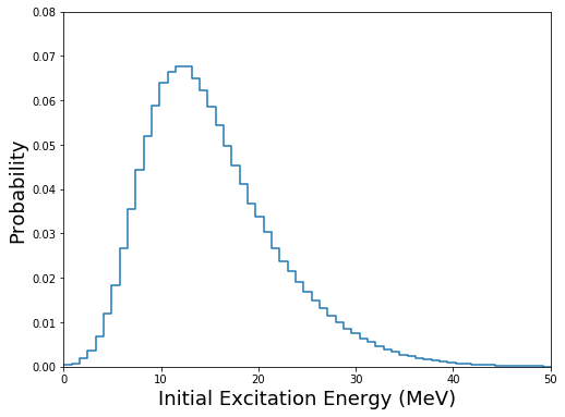
Manipulating and plotting those initial conditions can be done very simply with the help of numpy routines. For instance, finding the min, max, and mean values of the initial excitation energy in the fragments can be done by:

print (np.min(U), np.max(U), np.mean(U))

0.014787 82.1266 16.1717790934

and plotting the distribution of the excitation energy:

fig=figure(figsize(8,6))
h,b = np.histogram(U,bins=100,normed=True)
plt.step(b[:-1],h)
plt.xlim(0,50)
plt.xlabel("Initial Excitation Energy (MeV)",fontsize=18)
plt.ylim(0,0.08)
plt.ylabel("Probability",fontsize=18)
plt.show()

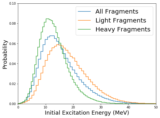
Separating the distributions for the light and heavy fragments can be done by recognizing that

Ul=U[::2]  # light fragments
Uh=U[1::2] # heavy fragments

fig=figure(figsize(8,6))
h,b = np.histogram(U,bins=100,normed=True)
hl,bl = np.histogram(Ul,bins=100,normed=True)
hh,bh = np.histogram(Uh,bins=100,normed=True)
plt.step(b[:-1],h,label="All Fragments")
plt.step(bl[:-1],hl,label="Light Fragments")
plt.step(bh[:-1],hh,label="Heavy Fragments")
plt.xlim(0,50)
plt.xlabel("Initial Excitation Energy (MeV)",fontsize=18)
plt.ylim(0,0.1)
plt.ylabel("Probability",fontsize=18)
lg=plt.legend(fontsize=20)
plt.show()

Similar plots and statistical analyses can be carried out for any initial quantity.